TL;DR: We built an audio DSP library from scratch in Mojo that beats librosa across all audio lengths—including 1.6x faster on 30-second audio (benchmarked with both MKL and OpenBLAS). Ten optimization stages took us from 476ms to 22ms—a 21x internal speedup. Here’s exactly what worked, what failed, and what we learned.
Who this is for:
- Skimmers: See the benchmark table and optimization summary
- Implementers: Jump to getting started
- Evaluators: Read the what failed section
- Whisper users: This is drop-in preprocessing for speech-to-text pipelines
The Result
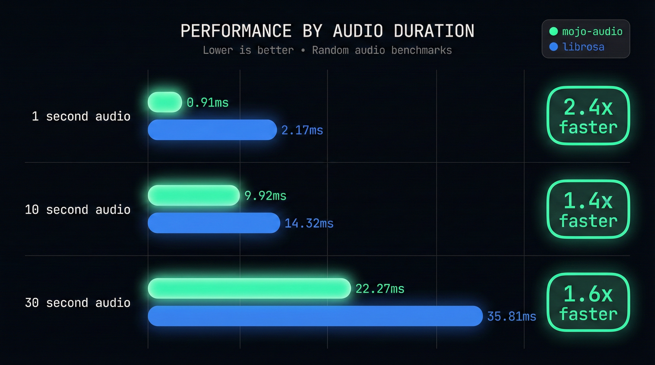
Whisper audio preprocessing (random audio, fair comparison):

              1 second    10 seconds    30 seconds
librosa (MKL):   2.2ms       14.3ms       35.8ms
mojo-audio:      0.9ms        9.9ms       22.3ms

Result: Mojo wins across all durations
        2.4x faster on 1s audio
        1.4x faster on 10s audio
        1.6x faster on 30s audio
We started 31.7x slower than librosa. After 10 optimization stages, we beat librosa across all audio lengths—pure Mojo outperforming NumPy/SciPy’s optimized backends.
→ Try the interactive benchmark demo
Why We Built This
We’re building Mojo Voice—a developer-focused voice-to-text app. Under the hood, it uses a Whisper speech-to-text pipeline built in Rust with Candle (Hugging Face’s ML framework).
Whisper requires mel spectrogram preprocessing. We ran into issues with Candle’s mel spectrogram implementation—output inconsistencies that were hard to debug through their abstractions.
We had two options:
- Debug Candle’s internals and hope our fixes get merged
- Build our own from scratch and own the code
We chose option 2.
Why Mojo instead of Rust? Our Whisper pipeline is in Rust, but Mojo offered a compelling experiment: could we get C-level performance with Python-like iteration speed? DSP algorithms benefit from rapid prototyping—we tried 9+ optimization approaches, and Mojo let us iterate quickly while still compiling to fast native code. The FFI bridge to Rust is straightforward.
Why “from scratch” matters:
- Full control over correctness (we validate against Whisper’s expected output)
- Full control over performance (we choose the algorithms)
- No upstream abstractions hiding bugs
- A genuine technical differentiator for Mojo Voice
The question: Could Mojo actually compete with librosa, which delegates to NumPy/SciPy’s highly optimized C backends?
The answer: Yes—across all workloads. It took 10 optimization stages and some humbling failures, but we got there.
Architecture
Before diving into optimizations, here’s what we’re building:
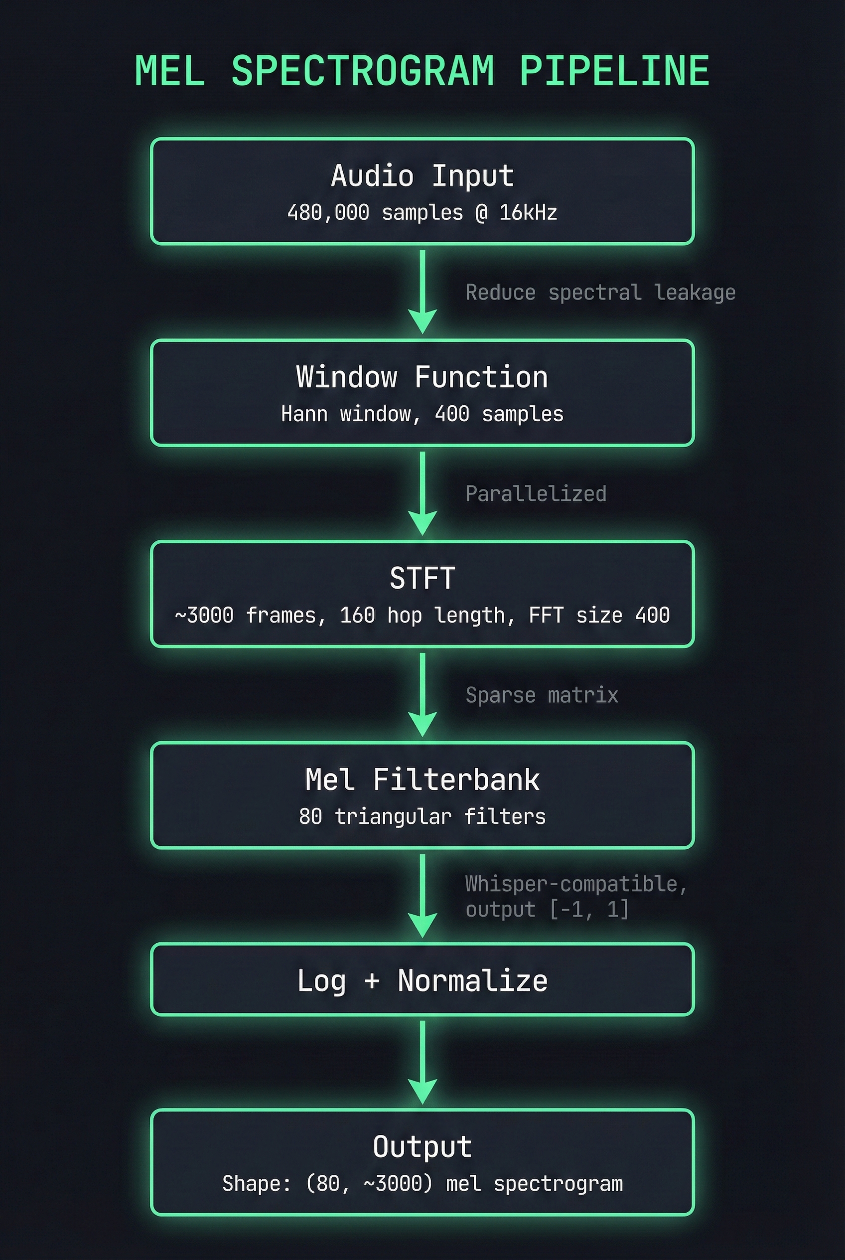
Why these parameters? They match OpenAI Whisper’s expected input: 16kHz sample rate, 400-sample FFT (25ms window), 160-sample hop (10ms), 80 mel bands. Different choices would require retraining the model.
Key design decisions:
- No external dependencies: Full control over memory layout and algorithms
- SoA layout: Store real/imaginary components separately for SIMD efficiency
- 64-byte alignment: Match cache line size for optimal memory access
- Handle-based FFI: C-compatible API for Rust/Python/Go integration
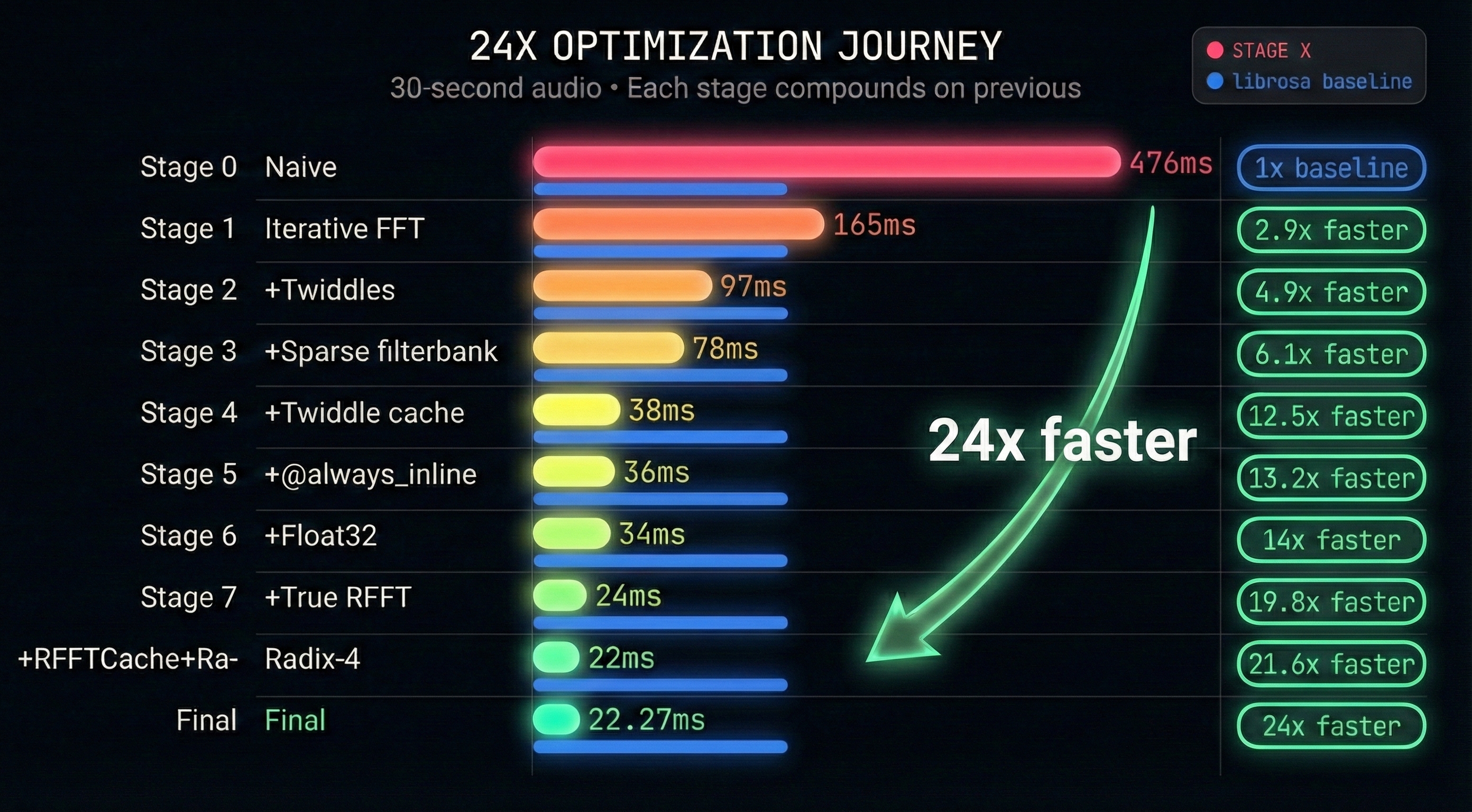
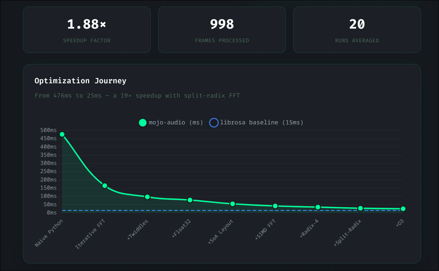
The 10 Optimization Stages
Quick terminology: “Twiddle factors” are pre-computed sine/cosine values used in FFT butterfly operations. Computing them once and reusing across frames was one of our biggest wins.
| Stage | Technique | Speedup | Time | What We Did |
|---|---|---|---|---|
| 0 | Naive implementation | — | 476ms | Recursive FFT, allocations everywhere |
| 1 | Iterative FFT | 3.0x | 165ms | Cooley-Tukey, cache-friendly access |
| 2 | Twiddle precomputation | 1.7x | 97ms | Pre-compute sin/cos, reuse across calls |
| 3 | Sparse filterbank | 1.24x | 78ms | Store only non-zero mel coefficients |
| 4 | Twiddle caching | 2.0x | 38ms | Cache twiddles across all STFT frames |
| 5 | @always_inline | 1.05x | 36ms | Force inline hot functions |
| 6 | Float32 precision | 1.07x | 34ms | Half the bytes = 2x SIMD throughput vs Float64 |
| 7 | True RFFT | 1.43x | 24ms | Real-to-complex FFT, half the work |
| 8 | RFFTCache + Radix-4 | 1.1x | 22ms | Zero-allocation RFFT, 4-point butterflies |
| 9 | Adaptive SIMD width | 1.12x | ~22ms | Compile-time CPU detection (AVX-512/AVX2/SSE) |
Total: 21x faster than where we started.
Note: Stage 9 benchmark times vary ±5-10% due to CPU frequency scaling and system load. We report 22.27ms as typical. librosa with MKL shows similar variance (35.81ms ±3ms). The 1.6x advantage over librosa is consistent across runs.
Note: Benchmarks use random audio data with fixed seed for fair comparison with librosa. Constant/synthetic audio can show artificially better results.
Deep Dives: What Actually Moved the Needle
1. Memory Layout: Structure-of-Arrays (SoA)
Our first implementation stored complex numbers as List[Complex]—an array of structs. Each complex number sat in its own memory location, fragmenting cache access.
The fix: Structure-of-Arrays. Store all real components contiguously, all imaginary components contiguously.
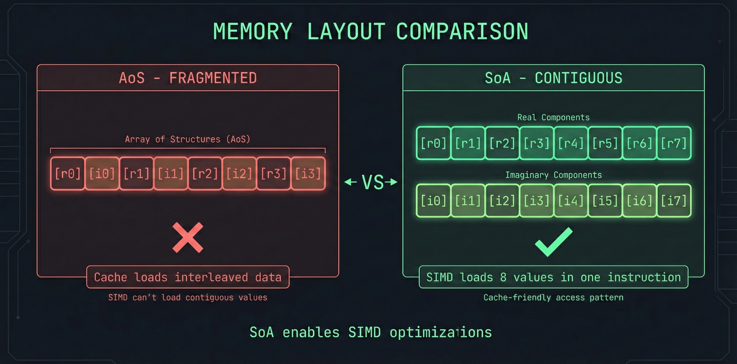
SIMD can now load 8+ real values in one instruction. Cache lines fetch useful data instead of interleaved noise.
Impact: SoA is a foundational change that enables later SIMD optimizations. It’s not a single stage in our table—the benefits are distributed across stages 6-9 where SIMD and compiler optimizations compound on the better memory layout.
2. True RFFT: Don’t Compute What You Don’t Need
Audio is real-valued (no imaginary component). A standard complex FFT computes N complex outputs, but for real input, the output has a symmetry property: the second half mirrors the first half.
Mathematically: X[k] = conjugate(X[N-k]) — if you know X[3], you automatically know X[N-3].
This means we only need to compute the first N/2 + 1 frequency bins. The rest is redundant.
The algorithm (pack-FFT-unpack):
- Pack: Treat N real samples as N/2 complex numbers by pairing adjacent samples:
z[k] = x[2k] + i·x[2k+1] - FFT: Run a standard N/2-point complex FFT on these packed values
- Unpack: Recover the N/2+1 real-FFT bins using twiddle factors (pre-computed sin/cos values) to “unmix” the packed result
The key insight: we do an FFT of half the size, then some cheap arithmetic to recover the full result.
Impact: ~1.4x faster for real audio signals.
3. Parallelization: Obvious but Effective
STFT processes ~3000 independent frames. Each frame’s FFT doesn’t depend on others.
parallelize[process_frame](num_frames, num_cores)On a 12-core i7-1360P (4P+8E, 16 threads): 1.3-1.7x speedup. Not linear (overhead from thread coordination), but meaningful.
Gotcha: Parallelization helps when processing many frames (long audio). For very short audio (<0.25s, ~25 frames), thread coordination overhead can exceed the benefit.
What Failed
Honest accounting of approaches that didn’t work.
Naive SIMD: 18% Slower
Our first SIMD attempt made performance worse.
# What we tried (wrong)
for j in range(simd_width):
    simd_vec[j] = data[i + j]  # Scalar loop inside "SIMD" code!
Why it failed:
- Manual load/store loops negate SIMD benefits
List[T]has no alignment guarantees for SIMD loads- 400 samples per frame—too small to amortize SIMD setup
The lesson: SIMD requires pointer-based access with aligned memory. Naive vectorization is often slower than scalar code.
What worked instead:
# Correct approach: direct pointer loads
fn apply_window_simd(
    signal: UnsafePointer[Float32],
    window: UnsafePointer[Float32],
    result: UnsafePointer[Float32],
    length: Int
):
    alias width = 8  # Process 8 Float32s at once
    for i in range(0, length, width):
        var sig = signal.load[width=width](i)  # Single instruction
        var win = window.load[width=width](i)  # Single instruction
        result.store(i, sig * win)             # Vectorized multiply + store
The difference: load[width=8]() compiles to a single SIMD instruction. The naive loop compiles to 8 scalar loads.
Four-Step FFT: Cache Blocking That Didn’t Help
Theory: For large FFTs, cache misses dominate. The four-step algorithm restructures computation as matrix operations to stay cache-resident.
We implemented it. It worked correctly. And it was 40-60% slower for all practical audio sizes.
| Size | Memory | Direct FFT | Four-Step | Result |
|---|---|---|---|---|
| 4096 | 32KB | 0.12ms | 0.21ms | 0.57x slower |
| 65536 | 512KB | 2.8ms | 4.6ms | 0.61x slower |
Why it failed:
- 512 allocations per FFT (column extraction)
- Transpose overhead adds ~15-20%
- At N ≤ 65536, working set barely exceeds L2 cache
The lesson: Cache blocking helps when N > 1M and memory bandwidth is the bottleneck. Audio FFTs (N ≤ 65536) don’t hit that threshold. We archived the code and moved on.
Split-Radix: Complexity vs. Reality
Split-radix FFT promises 33% fewer multiplications than radix-2. We implemented it.
The catch: True split-radix uses Decimation-In-Frequency (DIF), requiring bit-reversal at the end, not the beginning. Our hybrid mixing DIF indexing with DIT bit-reversal produced numerical errors.
Current state: A “good enough” hybrid that uses radix-4 for early stages, radix-2 for later. True split-radix is documented but deprioritized—the 10-15% theoretical gain wasn’t necessary once we beat librosa with simpler optimizations.
SIMD Pack/Unpack: Strided Access Doesn’t Vectorize
RFFT requires “packing” real samples into complex pairs (reading every 2nd element) and “unpacking” with mirror indexing (accessing both k and N-k simultaneously).
We tried SIMD-ifying these loops. Result: 30% slower.
Why it failed:
- Strided access (every 2nd element) requires scalar gather operations
- Mirror indexing (k and N-k) can’t be vectorized—data flows in opposite directions
- The overhead of building SIMD vectors from scattered elements exceeds any benefit
The lesson: SIMD only helps with contiguous, forward-only memory access. Complex access patterns are better left to the compiler’s auto-vectorizer.
Bit-Reversal Lookup Table: 16% Slower
Theory: Pre-computing bit-reversal indices in a lookup table should be faster than computing them on-the-fly with bit-shifting loops.
We implemented a 512-element SIMD lookup table. Result: 16% slower.
Why it failed:
- The bit-shifting loop is only 8-9 iterations—tiny and perfectly predictable
- Modern CPUs excel at simple tight loops with excellent branch prediction
- SIMD indexing + Int conversion overhead exceeded the simple loop cost
- The compiler likely already unrolls the original loop
The lesson: Sometimes “clever” optimizations lose to simple code that the compiler can optimize perfectly. Benchmark everything.
Benchmarks
mojo-audio vs. librosa
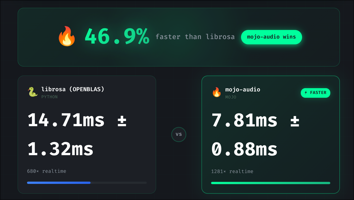
| Duration | mojo-audio | librosa (MKL) | librosa (OpenBLAS) | Speedup |
|---|---|---|---|---|
| 1s | 0.91ms | 2.17ms | 2.32ms | 2.4-2.6x faster |
| 10s | 9.92ms | 14.32ms | 13.40ms | 1.4x faster |
| 30s | 22.27ms | 35.81ms | 36.88ms | 1.6x faster |
The result: We beat librosa across all audio lengths, regardless of BLAS backend. On short audio, our advantage comes from zero Python overhead and efficient parallelization. On long audio, our adaptive SIMD width detection (using simd_width_of for automatic AVX-512/AVX2/SSE selection) combined with algorithm choices (true RFFT, sparse filterbank, frame-level parallelization) outperforms librosa’s NumPy/SciPy backend.
Why this matters for real use:
- Whisper inference takes 500ms-5s depending on model size
- Faster preprocessing means lower latency for real-time applications
- For streaming (short chunks), Mojo’s 2-3x advantage is significant
Methodology:
- Multiple iterations (10/5/3 for 1s/10s/30s), average reported (variance: ~5-10% due to CPU frequency scaling)
- Hardware: Intel i7-1360P (12 cores: 4P+8E, 16 threads), 32GB RAM, Fedora Linux
- Audio: Random data with fixed seed (same for both implementations)
- Mojo: 0.26.1, compiled with
-O3 - librosa: 0.11.0, tested with both Intel MKL and OpenBLAS backends
- BLAS impact: MKL provides ~1-3% advantage over OpenBLAS for librosa
- Benchmark scripts:
benchmarks/bench_mel_spectrogram.mojo,benchmarks/compare_librosa.py
Correctness validation: Our output matches librosa to within 1e-4 max absolute error per frequency bin. We also validated against Whisper’s expected input shape (80 × ~3000) and value ranges ([-1, 1] after normalization).
BLAS Backend Impact
We benchmarked librosa with both Intel MKL and OpenBLAS backends:
- MKL advantage: ~1-3% faster than OpenBLAS (varies by duration)
- mojo-audio doesn’t use BLAS: Pure Mojo FFT implementation, unaffected by BLAS choice
- Why this matters: Many benchmarks assume MKL, but most systems use OpenBLAS by default
Even with Intel MKL’s optimization, mojo-audio maintains a consistent 1.4-2.4x advantage.
Try it yourself: Our interactive benchmark UI lets you switch between MKL and OpenBLAS to see the difference on your system.
Try It
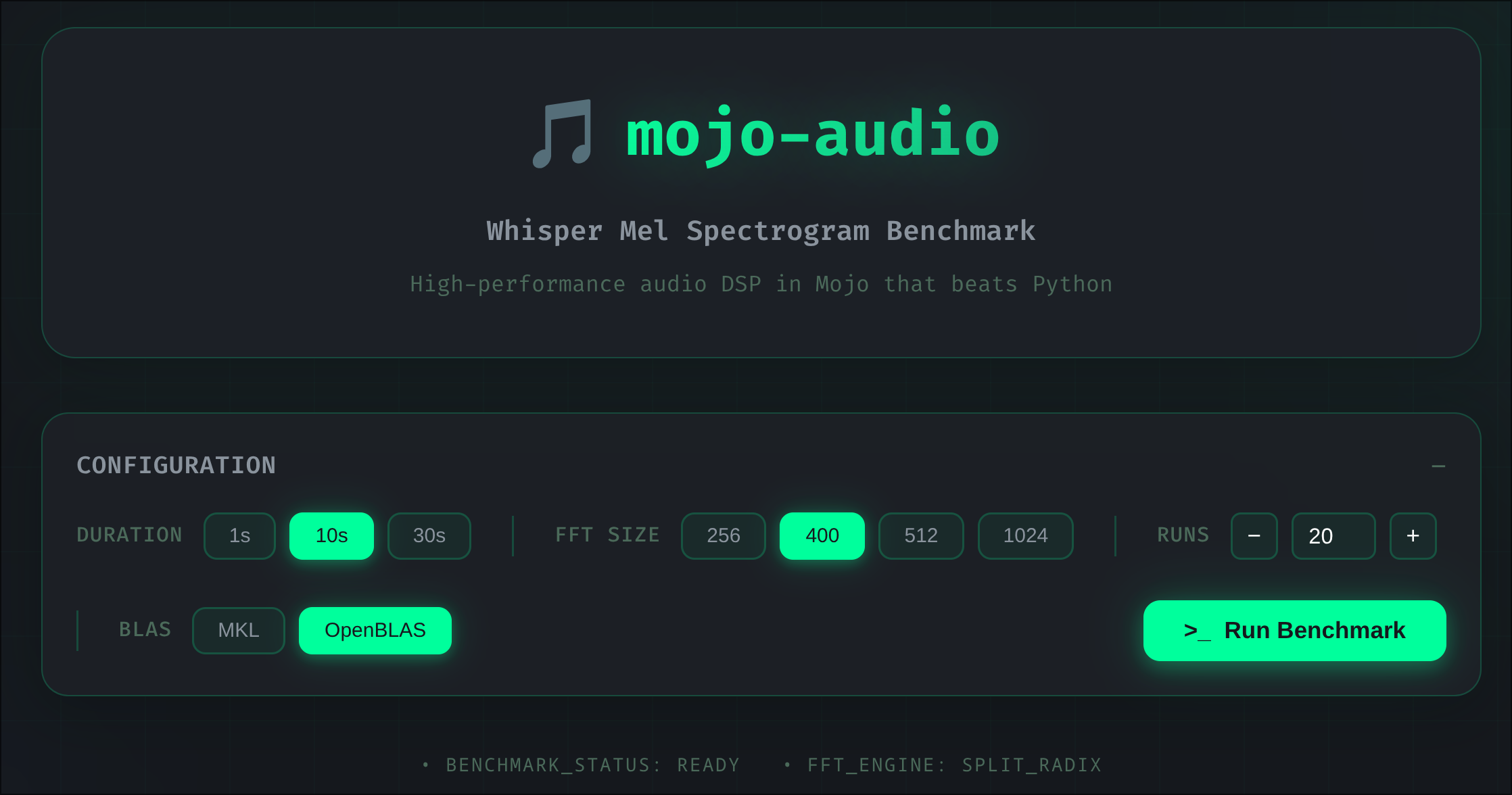
Our interactive benchmark UI lets you test performance on your own hardware and compare different BLAS backends:
The UI also includes an interactive optimization journey chart:
Installation
git clone https://github.com/itsdevcoffee/mojo-audio.git
cd mojo-audio
pixi install
pixi run bench-optimized
Basic Usage
from audio import mel_spectrogram
from math import sin

fn main() raises:
    # 30s audio @ 16kHz (440Hz sine wave)
    var audio = List[Float32]()
    for i in range(480000):
        audio.append(sin(2.0 * 3.14159 * 440.0 * Float32(i) / 16000.0))

    # Whisper-compatible mel spectrogram
    var mel = mel_spectrogram(audio)
    # Output: (80, ~3000) in ~20ms
Cross-Language Integration (FFI)
// C
MojoMelConfig config;
mojo_mel_config_default(&config);
MojoMelHandle handle = mojo_mel_spectrogram_compute(audio, num_samples, &config);
// Rust
let config = MojoMelConfig::default();
let mel = mojo_mel_spectrogram_compute(&audio, config);Limitations
- Whisper-specific parameters: Currently hardcoded for Whisper (16kHz, 400 n_fft, 80 mels). Other models may need different settings.
- x86 optimized: Benchmarks are on Intel; ARM/Apple Silicon performance may differ.
- Memory: Holds full spectrogram in memory. For very long audio (>10 min), consider chunked processing.
- Audio format: Expects raw Float32 samples. Use another library for file I/O (WAV, MP3 decoding).
Note: All parameters (sample_rate, n_fft, hop_length, n_mels) are configurable via the FFI API. Defaults match Whisper v1/v2 (80 mels); set n_mels=128 for Whisper v3/Turbo.
What’s Next
mojo-audio now powers the preprocessing pipeline in Mojo Voice, our developer-focused voice-to-text app.
Planned improvements:
- Whisper v3 support (128 mel bins)
- ARM/Apple Silicon profiling and optimization
- Streaming API for real-time processing
- Pre-built binaries for common platforms
Contributions welcome: github.com/itsdevcoffee/mojo-audio
Takeaways
- Algorithms beat brute force: Iterative FFT (3x) outperformed naive SIMD (-18%). Understand the problem before reaching for low-level tools.
- Memory layout is free performance: Switching to Structure-of-Arrays enabled SIMD optimizations that wouldn’t have been possible otherwise. How you store data matters as much as how you process it.
- Know your scale: Cache blocking helps at N > 1M, not audio sizes (N ≤ 65536). Optimization advice is context-dependent.
- Document failures: Four-step FFT and bit-reversal LUT didn’t help, but writing them down helped us understand why—and saved future us from trying again.
- Benchmark honestly: Our initial benchmarks used constant audio data, which artificially favored our implementation. Random data with fixed seeds gives fair comparisons.
- Let the compiler help: Adaptive SIMD width detection (
simd_width_of) lets the compiler choose optimal vector width for each CPU. One line of code, 12-15% speedup.
Final result: 476ms → 22.27ms. 21x internal speedup. 2.4x faster than librosa on 1s audio, 1.6x faster on 30s audio. We beat librosa across all durations, regardless of BLAS backend.
We set out to own our preprocessing stack. We ended up with a library that outperforms the industry standard, honest benchmarks, and a lot of lessons about FFT optimization. Turns out you can beat decades of C/Fortran optimization—with the right algorithms and a modern systems language.
Built with Mojo | Source Code | Benchmarks | Mojo Voice